This is an old revision of the document!
Table of Contents
Discs
These mock data are designed to mimic the Milky Way disc - either locally or globally. Key questions include, for the local problem:
(1) What quality of data are required to determine the local dark matter density? (2) Do multiple populations (e.g. split by abundance/age) help? (3) Is 1D modelling sufficient?
And for the global problem:
(1) Can global models simultaneously recover the disc phase space distribution function and the gravitational potential? (2) What are the key degeneracies in the problem and how can these be broken?
If posting new tests, please try to approximately follow the template set out for the “spherical collisionless tests” here.
Key working group coordinator: Daisuke Kawata
Local models/mocks
These mock data give positions and velocities for stars in and around the Solar neighbourhood, relevant for recovering the local Galactic potential and e.g. dark matter content.
Simple 1D data sampled from "Gaussian" Jeans equations
These first data assume a 1D population with zero “tilt” term. The velocities are sampled from the 1D vertical Jeans equation assuming Gaussian velocity distribution functions. This should be an easy test, but highlights:
- The importance of systematic errors due to over-restrictive assumptions about the potential;
- The role of sampling - i.e. how many stars are needed for what type of error;
- The importance of having different populations split by chemistry (and the errors introduced if we get this wrong);
- The importance of sampling high or low as compared to the disc plane; and
- The role of uncertainties in the baryonic mass model
We use a disc model:
<latex> \nu(z) = \exp(-z/z_0) </latex>
and vertical force law:
<latex> K_z = -\left[\frac{K z}{\sqrt{z^2 + D^2}} + 2Fz\right] </latex>
From which the vertical velocity dispersion (assuming no tilt) is:
<latex> \sigma_z^2(z) = \frac{1}{\nu(z)} \int_0^z \nu(z') K_z(z') dz' + \frac{C}{\nu(z)} </latex>
where <latex>C</latex> is a constant that sets the velocity dispersion at <latex>z = 0</latex>.
We set up several models as detailed in the following table:
| Model | Parameters | Data files | Plots | ||
|---|---|---|---|---|---|
| Simple | <latex>z_0 = 0.3\,{\rm kpc}</latex>; <latex>K = 1500</latex>; <latex>F = 267.65</latex>; <latex>C = 20 | 2</latex>; <latex>D = 0.18</latex>; <latex>n_* = 10 | 4</latex>; <latex>\Delta z_{\rm bin} = 0.05\,{\rm kpc}</latex> | simplenu_sigz_bin.dat simplenu_sigz.dat simplenu_sigz_raw.dat |  |
| Simplelow | As Simple, above, but with <latex>n_* = 10 | 3</latex> | simplelownu_sigz_bin.dat simplelownu_sigz.dat simplelownu_sigz_raw.dat | ||
| Simple2 | <latex>z_0 = 0.9\,{\rm kpc}</latex> and <latex>C = 40 | 2</latex>; otherwise as Simple, above | simple2nu_sigz_bin.dat simple2nu_sigz.dat simple2nu_sigz_raw.dat |  | |
| High | As Simple2, above, but with <z_0 = 1.5\,{\rm kpc}</latex>; data cut on 2 < z < 4 kpc; just 500 stars; and <latex>\Delta z = 0.25\,{\rm kpc}</latex> | highnu_sigz_bin.dat highnu_sigz.dat highnu_sigz_raw.dat |  |
where <latex>n_*</latex> is the number of stars, and <latex>\Delta z_{\rm bin}</latex> is the bin size (for the binned data).
The data files are as follows:
- simplenu_sigz_bin.dat :: Binned data: <latex>z [{\rm kpc}], \nu(z), \nu_{\rm err}(z), \sigma_z(z) [{\rm km/s}], \sigma_{z,{\rm err}}(z)</latex>
- simplenu_sigz.dat :: Smooth model
- simplenu_sigz_raw.dat :: Raw particle data in <latex>[z,v_z]</latex>
- simple.png :: Plots of the above.
The system of units is kpc, Msun, km/s. Converting the vertical force to a surface density (<latex>M_\odot\,{\rm kpc}^{-2}</latex>) via the Poisson equation (assuming no rotation curve contribution), we have:
<latex> \Sigma_z(z) = \frac{|K_z|}{2\pi G_1} </latex>
where:
<latex>G_1 = 6.67 \times 10^{-11} \times 1.989\times 10^{30} / 3.086\times 10^{19}</latex>
Results so far
Simple code by Justin Read. Preliminary: adventures.pdf.
Global models with known background potential
N-body disc models simulated with GCD+ (Kawata & Gibson 2003). These are the target disc models used in Hunt, Kawata & Martel (2013). The fixed Navarro, Frenk & White (1997) dark matter halo profile is applied:
<latex>\rho _{dm}=\frac{3H_{0}^{2}}{8\pi G}\frac{\Omega _{0}-\Omega_b}{\Omega_0}\frac{\delta_{c}}{cx(1+cx)^{2}}</latex>
where:
<latex> c=r_{200}/r_s </latex>,
<latex> x=r/r_{200},</latex>
<latex>r_{200}=1.63\times 10^{-2}\left(\frac{M_{200}}{h^{-1}M_{\odot}}\right)^{\frac{1}{3}} h^{-1},</latex>
and:
<latex>\delta_c = \frac{200}{3} \frac{c^3}{\left[\ln(1+c) - c/(1+c)\right]}.</latex>
We assume <latex>\Omega_0=0.266=1-\Omega_{\Lambda}</latex>, <latex>\Omega_{\rm b}=0.044</latex>, and <latex>H_0=71{\rm kms^{-1}Mpc^{-1}}</latex>. A live N-body disc is initially set up and simulated for several Gyr. The data file provides the position, velocity and mass of the disc particles. If you have any question, please email d.kawata (at) ucl (dot) ac (dot) uk.
ASCII data file format:
x,y,z,vx,vy,vz,mp
… format(7(1pE13.5))
x,y,z … position (kpc)
vx,vy,vz … velocity (km/s)
mp … particle mass (Msun)
| Model | Description | <latex>M_{200}/M_\odot</latex> | <latex>c</latex> | <latex>N</latex> | Data file | Plot |
|---|---|---|---|---|---|---|
| GD1 | Smooth disc | 1.75e12 | 20 | 99,9982 | gcdpdnf1.dat.gz |  |
| GD2 | Barred disc | 2.0e12 | 9 | 1,000,000 | gcdpdbar1.dat.gz |  |
Error added data
Additionally, we provide the target GD2 in equatorial coordinates, with and without a Gaia-type error, treating the particles as tracers for a single stellar population, in this case M0 Giants.
The errors are computed following Gaia science performance estimates (credit to Mercè Romero Gómez & Francesca Figueras.)
The sun is located at (-8,0,0) kpc in cartesian coordinates. (Note that this does not take into account extinction)
ASCII data file format and units:
output.txt
| Model | Description | <latex>M_{200}/M_\odot</latex> | <latex>c</latex> | <latex>N</latex> | Data file |
|---|---|---|---|---|---|
| GD2 | M0 tracer Barred disc w & w/o error | 2.0e12 | 9 | 1,000,000 | ubgaiae-out.dat.gz |
| GD1 | Smooth Red Clump w & w/o error | 1.75e12 | 20 | 999,987 | rc-out.dat.gz |
| GD2 | barred Red Clump w & w/o error | 2.0e12 | 9 | 1,000,000 | rc-bar.dat.gz |
For the GD1-RC stars for the challenge, the velocity of the sun w.r.t the GC is (0, 228.14, 0) km/s with the sun again at (-8,0,0) kpc.
Publication policy
If using these test data, please cite the Gaia Challenge wiki and Hunt, Kawata & Martel (2013).
Challenge
- First simple challenge can be recovering the surface density profile, mean rotation velocity profile and velocity dispersion profile as a function of radius from a partial data (e.g. using the particle data within 10 kpc from (x,y,z)=(-8,0,0) kpc.
- Recovering the surface density profile, mean rotation velocity profile and velocity dispersion profile as a function of radius from the error added data.
Test Results
This section can be used to post test results from applying your method(s) to the above test data. There is no obligation to post data here, but this area could form the basis of a publication writing up our first “Gaia Challenge” findings.
PRIMAL applied to the suggested challenges
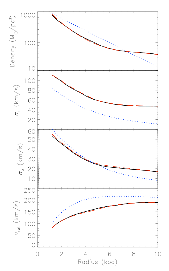
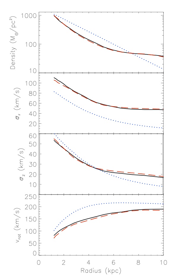
To start things off, we show the results of our Particle-by-particle M2M algorithm (PRIMAL) when applied to the barred galaxy target above with and without error. We start from a smooth disc with a different scale length, and recover the target while using the 10 kpc sphere of observation around the sun as suggested above.
Without error, it is easy to recover the radial profiles for the density, radial and vertical velocity dispersions, and the mean rotational velocity form the partial data. See Fig. 1, the black solid line is the target, taken from the complete data, the blue dotted line is our starting point, and the red dashed line is our final model. As you can see this produces a very good fit (as shown in Hunt, Kawata & Martel (2013)).
With error however things become more difficult. As a work in progress we are modifying PRIMAL to work with data containing error, and we show our best attempt so far in Fig. 2. We are happy with the density profile but we are continuing to make improvements to the algorithm to allow us to better recover the velocity profiles.
Challenge A (see below)
Bovy
See his presentation
K$_{z,1.1}$ is similar to the target galaxy.
Chemin
See his presentation chemin-gaiachallenge.pdf
Recover rotation curve and pattern speed of the bar and spirals.
Analytic global models with a known distribution function and background potentials
N-body representations of an analytical distribution function of the form used by McMillan and Binney (2012), evaluated in two different potentials. The distribution function represents a single “pseudo-isothermal” disc in each potential. The potentials are Milky Way-like and constructed from several spheroidal and disc like components (as in McMillan 2011).
The particles are tracers (zero mass), and the data files provide their exact positions and velocities (x,y,z,vx,vy,vz) in units of kpc and kpc/Myr (1 kpc/Myr = 977.775 km/s). Questions or comments to p.mcmillan1 (at) physics (dot) ox (dot) ac (dot) uk.
Data file 1 from first potential.
Data file 2 from second potential.
Analytic models with known df - Red Clump test
Again, N-body representations in the same two potentials - the distribution function is slightly more complicated. Data represent red clump stars (all having intrinsic G=1, V-I=1), with data including uncertainties as per those expected from Gaia, so if G>16, the radial velocity is unknown (N.B. unknown radial velocities are quoted as 0 with uncertainty given as -1)
Data format: gzipped space separated ascii, with explanation in header line (behind a # symbol):
RA(radians) dec(radians) true_parallax(mas) true_mu_a*(mas/yr) true_mu_d(mas/yr) true_vr(km/s) RA(radians) dec(radians) obs_parallax(mas) obs_mu_a*(mas/yr) obs_mu_d(mas/yr) obs_vr(km/s) err_parallax(mas) err_mu_a*(mas/yr) err_mu_d(mas/yr) err_vr(km/s) abs_G obs_G x(kpc) y(kpc) z(kpc) vx(km/s) vy(km/s) vz(km/s)
(78 Mb each, Data file 1b Data file 2b)
The Sun is placed at x=8kpc, y=0, z=0. The Sun's velocity with respect to the Galactic Centre is vR = -11.1 km/s, vz = 7.25 km/s and vphi = -258.7 km/s for model H or -249.5 km/s for model G.
Publication policy
If using these test data, please cite the Gaia Challenge wiki and McMillan and Binney (2012).
Challenge
A challenge remains to be defined for these data.
Full N-body models (with local cuts)
These are full collisionless N-body simulations. The first two were published and analysed in http://adsabs.harvard.edu/abs/2011MNRAS.416.2318G and http://adsabs.harvard.edu/abs/2012MNRAS.425.1445G. The latter two include a perturbing satellite at low and high inclination and will be published shortly in Read et al. 2013 in prep.
There are four simulations:
Each .tar bundle contains:
- densityfalloff_dm/stars :: ASCII file data for the dark matter/star density fall-off at different radii and angle for small volumes around the disc.
- surfacedensity_bar/dm :: As above for the surface density for the baryons and dark matter.
- velocity dispersion :: As above for the stellar velocity dispersion in the z-direction (perpendicular to the disc).
- wedges :: Raw unbinned ASCII data for different wedges cut around the disc as in http://adsabs.harvard.edu/abs/2011MNRAS.416.2318G.
- *.txt.gz :: Raw ASCII data for the entire centred and aligned simulations (excluding the accreted satellite stars and dark matter). Warning: These files are large (>2 GB).
Publication policy
If using these test data, please cite the Gaia Challenge wiki, http://adsabs.harvard.edu/abs/2011MNRAS.416.2318G, and Read et al. 2013 in prep.
N-body models from Elena D'Onghia
Snapshots provided by Elena D'Onghia from her simulations in http://adsabs.harvard.edu/abs/2013ApJ...766...34D, which have 100 million disk particles. Ask Jo Bovy to get these from a USB stick. The simulation and data consists of snapshots at 0 Myr (initial conditions), 250 Myr, and 1 Gyr (snap_000.hdf5, snap_005.hdf5, snap_020.hdf5).
The galaxy model consists of an Hernquist halo with total mass of 9.5×10^11 Msun computed at a radius of 160 kpc. The halo is simulated with a rigid potential. The concentration of the halo is adopted to be c=9 for an Hernquist profile which is approximately like c=12 for a NFW profile. The spin parameter of the halo is lambda=0.033. This galaxy contains a live stellar disk and a little live bulge that made more stable the disk:
Disk:
The disk fraction is: Mdisk/Mhalo=0.04 The scale length is 2.5 kpc. We introduced perturbers corotating with the stellar disk as softened particles (the total number of perturbers is 1000 and each has a mass of 9.5×10^5 Msun so that the total mass of the perturbers is ~ 9.5×10^8 Msun which is ~2.5% of the total disk mass). In the run we fixed the softening of the perturbes with size of giant a molecular cloud: ~100 pc. In the initial setup the vertical thickness of the disk is setup z0=0.1 of the scale length. Number of particles in the disk= 100 millions. In gadget snapshot stellar disk particles are type 2.
Bulge:
The bulge fraction is: 0.01. The size is 0.1 of the disk scale length. Number of particles in the bulge is : 10 millions. In gadget snapshot bulge particles are type 3.
The particles that mimic the perturbers are 1000 and in gadget are type 4.
Q parameter is initially set up to be larger than 1.3 at all radii.
Publication policy
If using these test data, please cite the Gaia Challenge wiki and http://adsabs.harvard.edu/abs/2013ApJ...766...34D.
Test particles data (Barred potential)
Data provided by UB team (Romero-Gomez et al.). The simulation is described here.
Ascii file: 21635205 Red Clump particles with Grvs<16.1 (from a sample of 72M)
-In each row:
G ,Grvs ,Xreal (Kpc),Yreal (Kpc),Zreal (Kpc),VXreal (Km/s),VYreal (Km/s),VZreal (Km/s),Xobs (Kpc),Yobs (Kpc),Zobs (Kpc), VXobs (Km/s),VYobs (Km/s),VZobs (Km/s)
-Positions and velocities are galactocentric. -The Sun is placed at (-8.5,0,0)Kpc
-data format: (2(f7.3,1x),3(f7.3,1x),3(f10.2,1x),3(f7.3,1x),3(f10.2,1x))
-Real values = without errors -Obs values = with Gaia errors
Also available (not in the ascii file):
-Av ,V ,V-I ,GL ,GB ,dist ,xmuls ,xmub ,VR ,GLOBS ,GBOBS ,distobs ,xmulsobs ,xmubobs ,VROBS ,sigalpha ,sigdelta ,sigpi ,sigmua ,sigmud ,sigvr
-The full sample without the cut at Grvs<16.1
The simulation data is too large to upload it to the twiki. We can provide it in a USB stick or you can find it at google drive: https://docs.google.com/file/d/0B8sgZGL4aKpSc3dlUnRKdkszaHM/edit?usp=sharing .
Results
Challenge B (see below)
Input bar pattern speed: $\Omega_p=50$ km/s/kpc
Monari
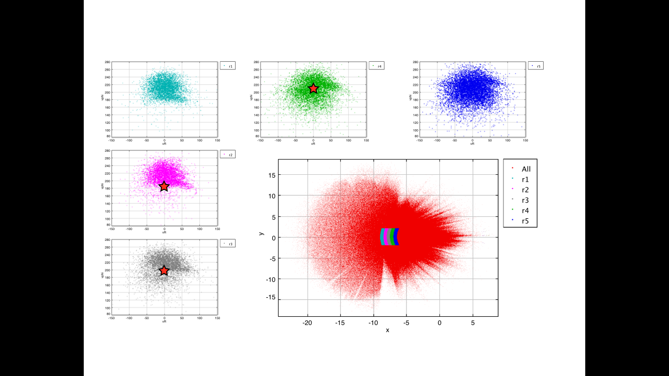
V$_{\phi}$ vs. V$_R$ map at the various location, and looking for OLR feature.
 Using flat circular velocity curve model (v0), and $\Omega_p$ as free parameters I get $v0\sim210$ km/sec and $\Omega_p\sim$50km/sec/kpc, with and without errors, nearby the Sun.
Pfenniger
- Based on the usual Fourier decomposition in rings
- Based on moment of inertia
- (semi-local TW method)
Conclusion: a not too wrong value 35-42 [km/s/kpc] is found around 4-5 kpc, with a systematic lower value for the data with noise in both the moment of inertia and the Fourier methods. However, the inner (0-2 kpc) values are very noisy, and no obvious plateau in R is found.
Victor Debattista's Model R1
This is the Milky Way scaled version of Model R1 of http://adsabs.harvard.edu/abs/2005ApJ...628..678D, which is selected one of the best Milky Way model in http://adsabs.harvard.edu/abs/2013arXiv1306.4694G.
| Model | Description | Data file |
|---|---|---|
| Moderl R1 | Barred N-body simulation | http://www.star.uclan.ac.uk/~vpd/modelR1GaiaChallenge.gz |
Publication policy
If using these data, please cite the Gaia Challenge wiki and Debattista et al. (2005) and Gardner et al. (2013).
Discussion on 19-23 Aug, 2013
These are ideas and initial results of the challenges discussed in the Surrey workshop week. However, please feel free to post your mock data, grab the data and do your own challenge. Please also feel free to discuss off-line and build up collaborations.
Aim:
Sharing the mock data.
Comparison among different dynamical modelling methods using various mock data.
Challenge A:
Who expressed their interests in participating
Bovy, McMillan, Chemin, Hunt, Buedenbender, Sharma, Roca-Fabrega, Monari, Inoue, Read, Steger
Challenge
deriving 3D force fields from the mock data: measure force in 3D, F$_R$, F$_{\phi}$, F$_z$ as a function of R, $\phi$, z grid points
Grid
Grid in Galactic R, $\phi$, z
R: 3-20 kpc in radius
|z|: 0-4 kpc
$\phi$: +-45 deg (for Paper 1 below, no $\phi$ grid)
whoever got the first results can decide bin size.
mock data:
Smooth disc: McMillan model
Smooth N-body simulation: GD1 (1M particles, see above), D'Onghia disk (100 M)
input data:
- heliocentric equatorial coordinate: R.A. DEC, parallax, proper motion (mas/yr), radial velocity (km/s)
- position and motion (w.r.t. GC) of the Sun (R$_{Sun}$=8 kpc, z=0)
- selection function
- RC tracer, solar metallicity with and without Gaia error G < 20.
- Use radial velocity data for only G_RVS < 17
- RC stars: M_G=1 mag, V-I=1.0, sig M_G=0
- no extinction
data format:
ascii data
Results
Challenge B:
Who expressed their interests in participaiting
Pfenniger, Monari, Hunt, Roca-Fabriga, Chemin
Challenge
Recovering the pattern speed of the bar.
Mock Data
N-body Barred galaxy
-GD1 (Hunt)
-Debattista bar model
UB Test particle simulation with a bar potential
Input Data
* RC tracers
* with or without Gaia error
* with or without extinction
Challenge C:
1D vertical force field reconstruction
Future
Cosmological simulations, multiple populations, dust extinction
Appendix:
Mock data available?
Cosmological simulations:
N-body+gas:
N-body: smooth, structured, barred, multi-compents, bulge
Test particles: bar potential, spiral arms
Analytic: smooth disk
Galaxia:
GUMS: kinematic model, multiple populations, dust extinction
Challenges: what we want to analysis?
starting: GD1 without error
selection function - cutting within sphere - cutting |z|<1~0.1 kpc - known dust extinction
- - smooth disk exponential
- - Schlegel(?) map, Galaxia type dust
- - 3D extinction
- multiple populations
- Who is interested in what?
L. Chemin … derive rotation curve, DM vs. disk potential. Location of bar, resonance.
P. McMillan … N-body with error, the local+whole potential
S. Roca-Fabrega … Moment of distribution function, vertex deviation, bar pattern speed, spiral arm (number) position and perturbation
J. Bovy … vertical force.
J. Hunt … M2M modelling. disc structure, DM potential?
S. Sharma … analysing rotation curve
S. Inoue … vertical disc structure, local DM density
G. Monari … velocity distribution, local and radial gradient, with structures
Read/Steger … vertical force; local DM density


